3DOptix User Guide v. 1.1
Table of Contents
3DOptix is an online software package for optical design and ray optics simulation.
The unique 3DOptix ray-tracing engine runs in the cloud and is accessible via any browser. The tool is very intuitive and enables you to quickly plan and test any optical setup with off-the-shelf optomechanics, common light sources and a very wide variety of optical elements from a number of leading vendors, as well as your own customized optics solutions.
This user guide explains in detail how to work with 3DOptix.
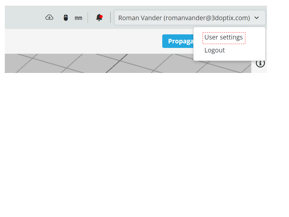
shows mouse controls
presents the metrics unit for this setup
opens the Notification Center
Undo/Redo
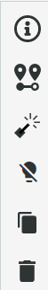
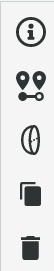
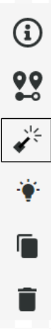
By selecting any element on the layout or in the Outliner, a corresponding toolbar is opened in the top right corner of the screen. See below from left to right for light source, optical elements and detector. There are common features, such as - Part information, - Move/rotate, - Duplicate and - Delete, and element type specific features: - Light source settings, - Light off, - Optics settings and Detector element.
The Outliner appears on the left side of the screen.. It can be minimized or maximized by clicking these buttons. The Outliner shows all the objects in the setup, their surfaces and local coordinate systems (LCS). Please note that surfaces and LCS can be selected from the Outliner as well as on the layout. The Global Coordinate System (GCS) is the first entity in the Outliner.
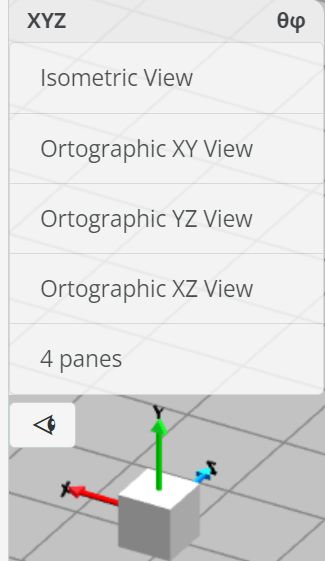
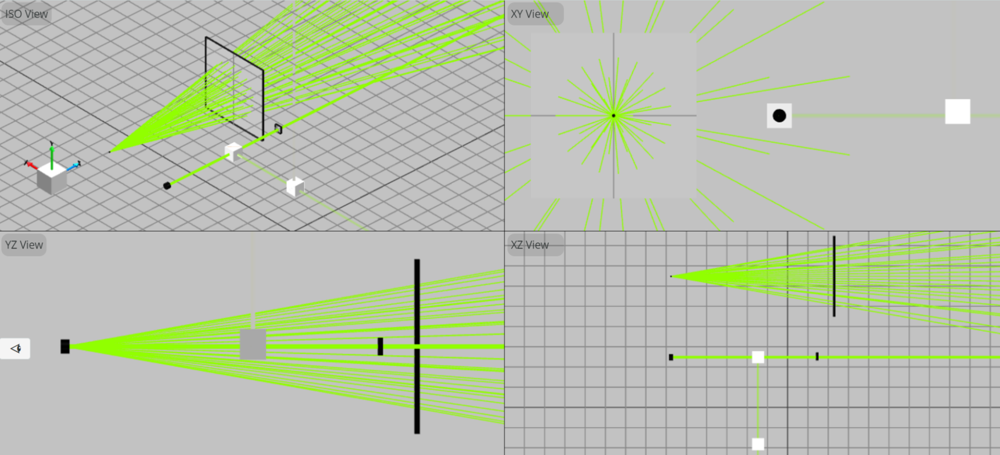
The setup can be viewed in the isometric view or one of the orthographic views by clicking , or alternatively clicking on “4 panes” which will show all views on a single screen. Double-clicking on one of them turns the mode into a single pane, showing the clicked view.
A Global Coordinate System (GCS) is located at (x,y,z) = (0,0,0). The GCS serves as a default coordinate system for newly added elements.
Each newly added element is positioned relative to the GCS, according to the position of the mouse cursor. The breadboard plane is defined as y = 0 height. The default for a new element is y = 10 mm, in order to locate the element above the breadboard.The element can then be precisely positioned and rotated using the Move/rotate feature.
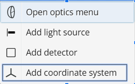
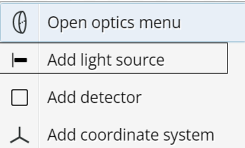
Each element surface has its own Local Coordinate System (LCS) attached to it. When elements are positioned relative to each other, the linkage is done by LCS. You can add an LCS in the same way that elements are added: right click and select Add coordinate system.
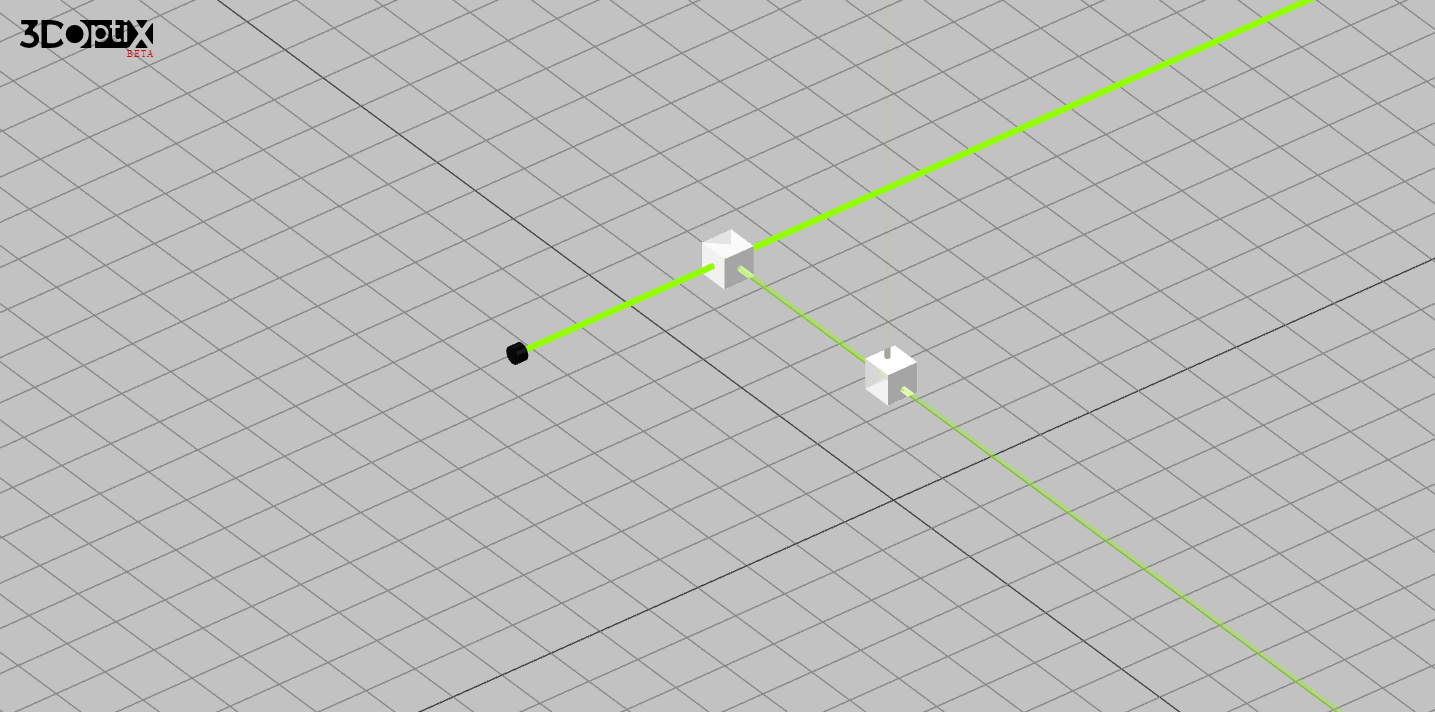
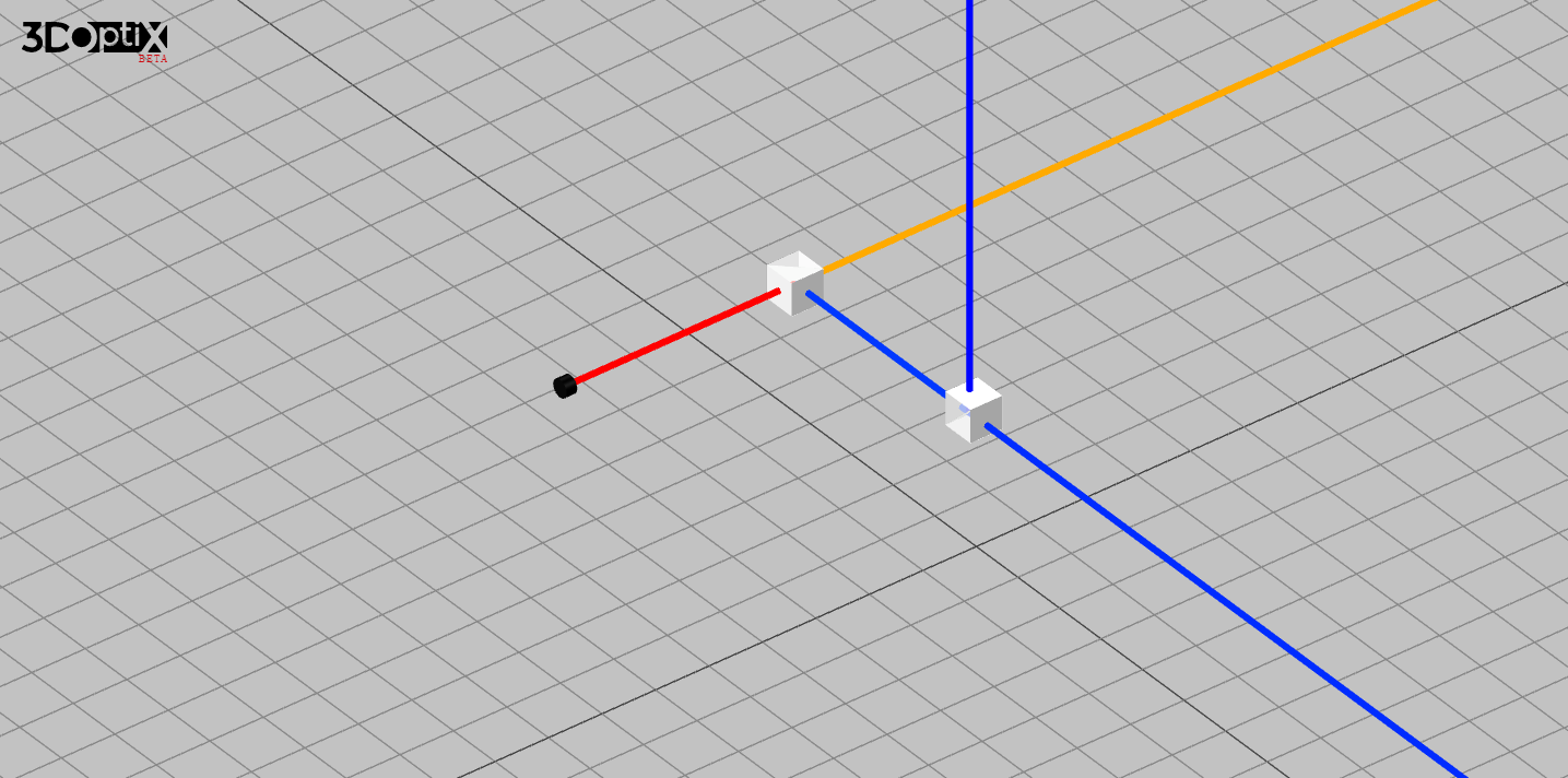
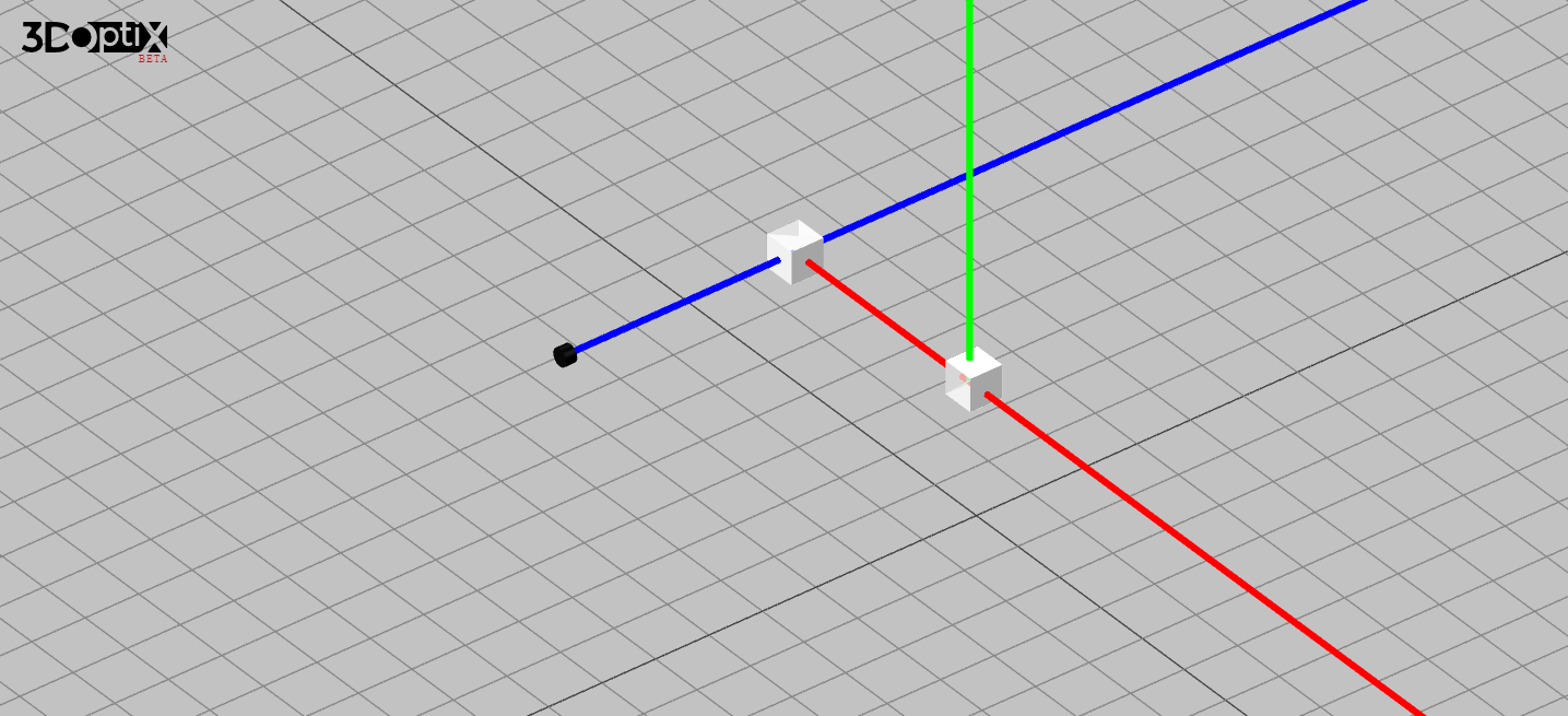
Ray Color Palette Example
The same setup consisting of a collimated single wavelength source incident on two T:R= 70:30 beam splitters is shown below in each of the three color palette modes.
Spectral Color Mode
Intensity Color Mode
Directional Color Mode
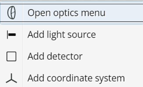
At the approximate desired location, right-click Add light source.
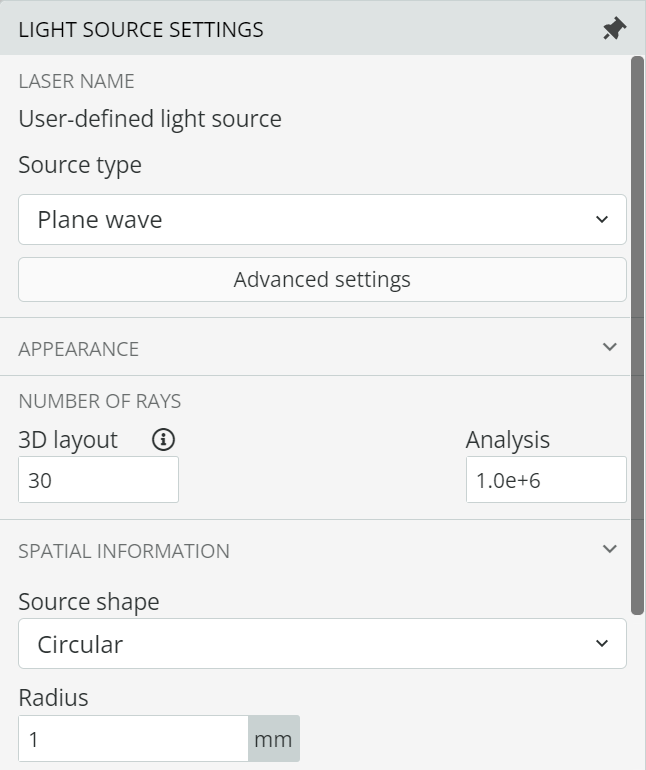
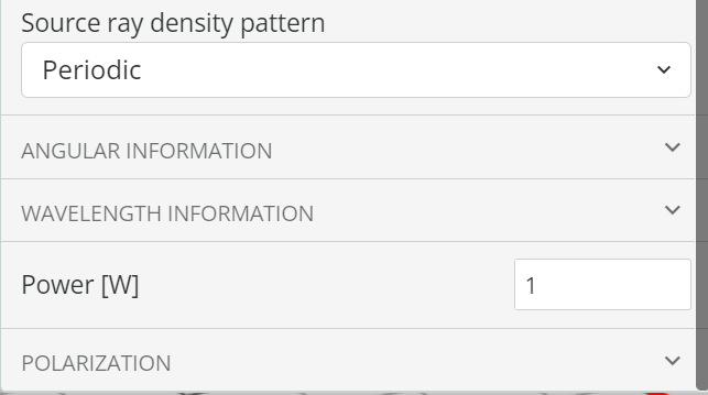
The light source is added to the layout. The default light source is plane wave. You can modify the default parameters by clicking on the layout or selecting the parameter from the Outliner on the left side. The right toolbar will appear. Click the Light source settings button to open this dialog box:
For each distribution type (except user-defined) select 𝝺min, 𝝺max, 𝚫 (step or increment) and then click the Apply button. 3DOptix automatically creates wavelengths with the appropriate weights, according to the selected distribution type. In the user-defined type, manually add the wavelengths and specify their weights. Note: The first in the list wavelength (with a non-zero weight) for TH distribution, or peak wavelength for the Blackbody and Gaussian types, is marked “primary”, though you can change this. The primary wavelength is used for calculations and cannot be deleted.
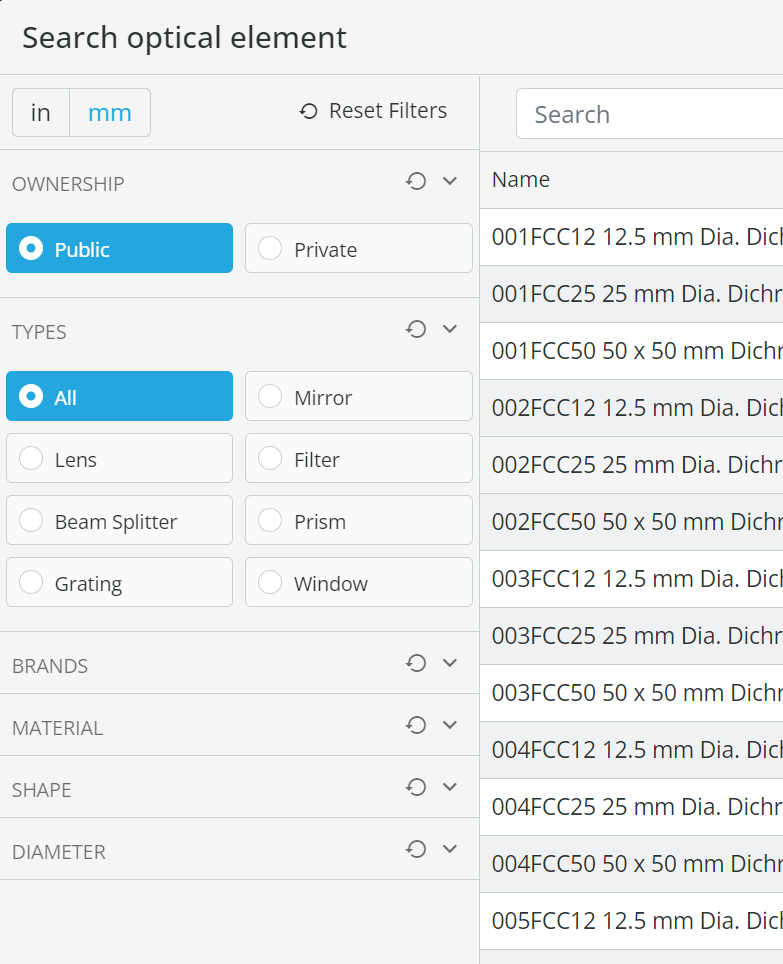
At the approximate desired location, right-click Open optics menu.
The Search Optical Element window opens. There are two ways of searching in the 3DOptix library:
After applying filters, click a result and the element will be placed at the cursor location.
Click the button on the right toolbar to open the Element Settings window where you can see and change (in some cases) the element parameters. There is a link to the vendor page and a 3D image of the element is displayed.
Element Settings

 - Intensity in the
  direction.
 - Intensity in the specular direction.
 - azimuthal scatter angle measured from the local x-axis.
 - standard deviation of the Gaussian distribution parallel the local x-axis.
 - standard deviation of the Gaussian distribution parallel the local y-axis. - polar angle.
 - Intensity in the direction. - Intensity in the specular direction. - polar angle.
 - Intensity in the direction. - Intensity in the specular direction. - polar angle.
 - distribution parameter.
 - polar angle of scattering distribution.


 - scattering parameter.
Click thebutton on the Outliner to add an opto-mechanical component. Select the part using the search window or filter by vendor or type. The proposed parts are displayed and can be dragged to the layout. In a future release there will be an opto-mechanics search portal, similar to the optics search portal
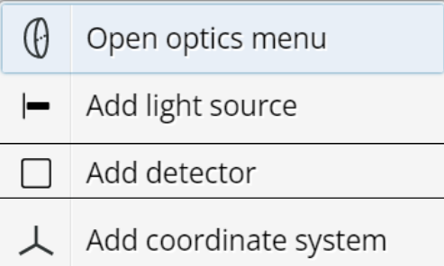
At the approximate desired location, right-click Add detector.
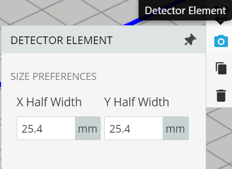
A 50.8 mm x 50.8 mm default detector is added to the layout. Click the detector to modify the default parameters or select it from the Outliner on the left side. In the right toolbar that appears, click the Detector element button to modify the detector size (X Half Width and Y Half Width) can be modified.
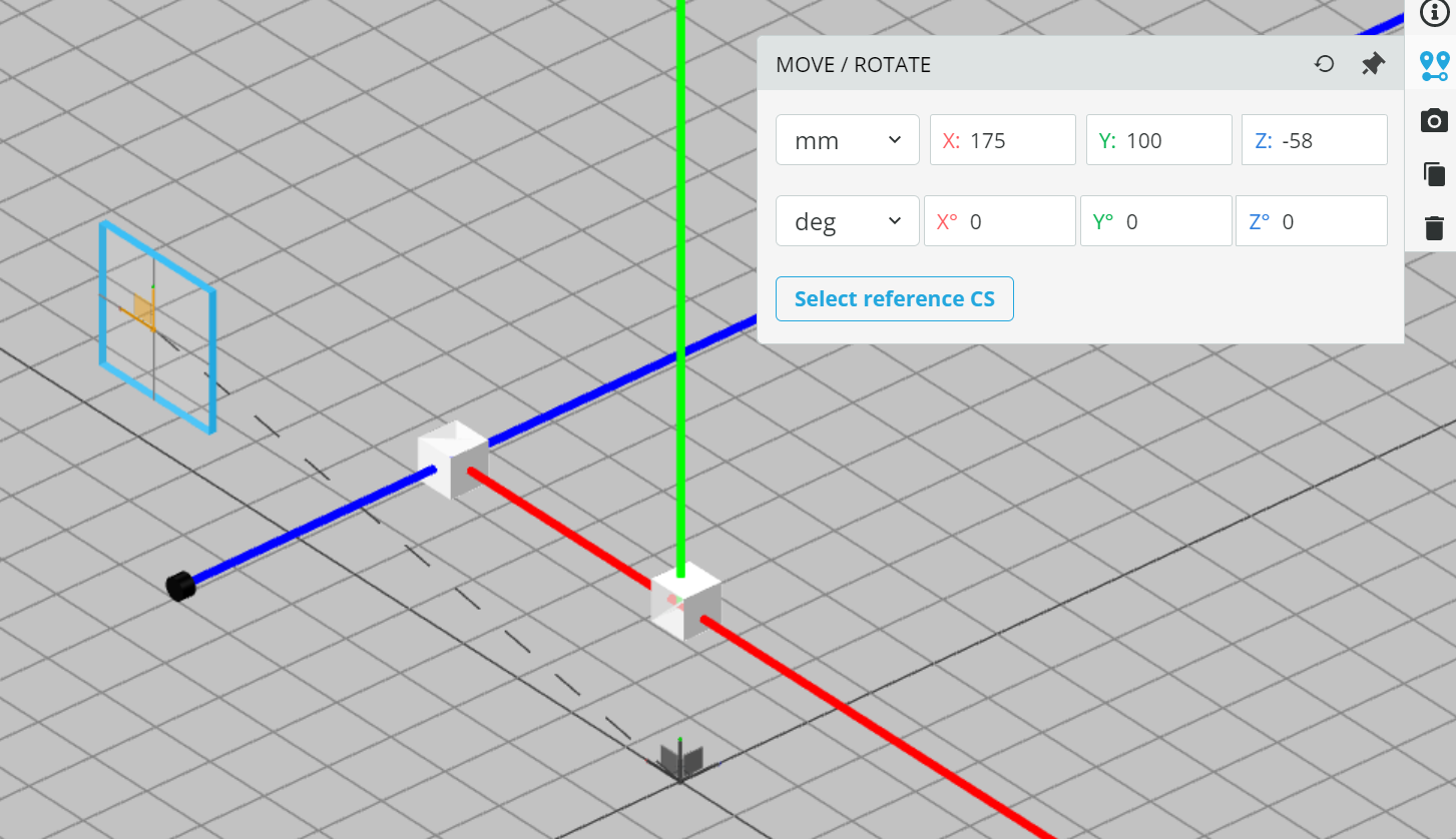
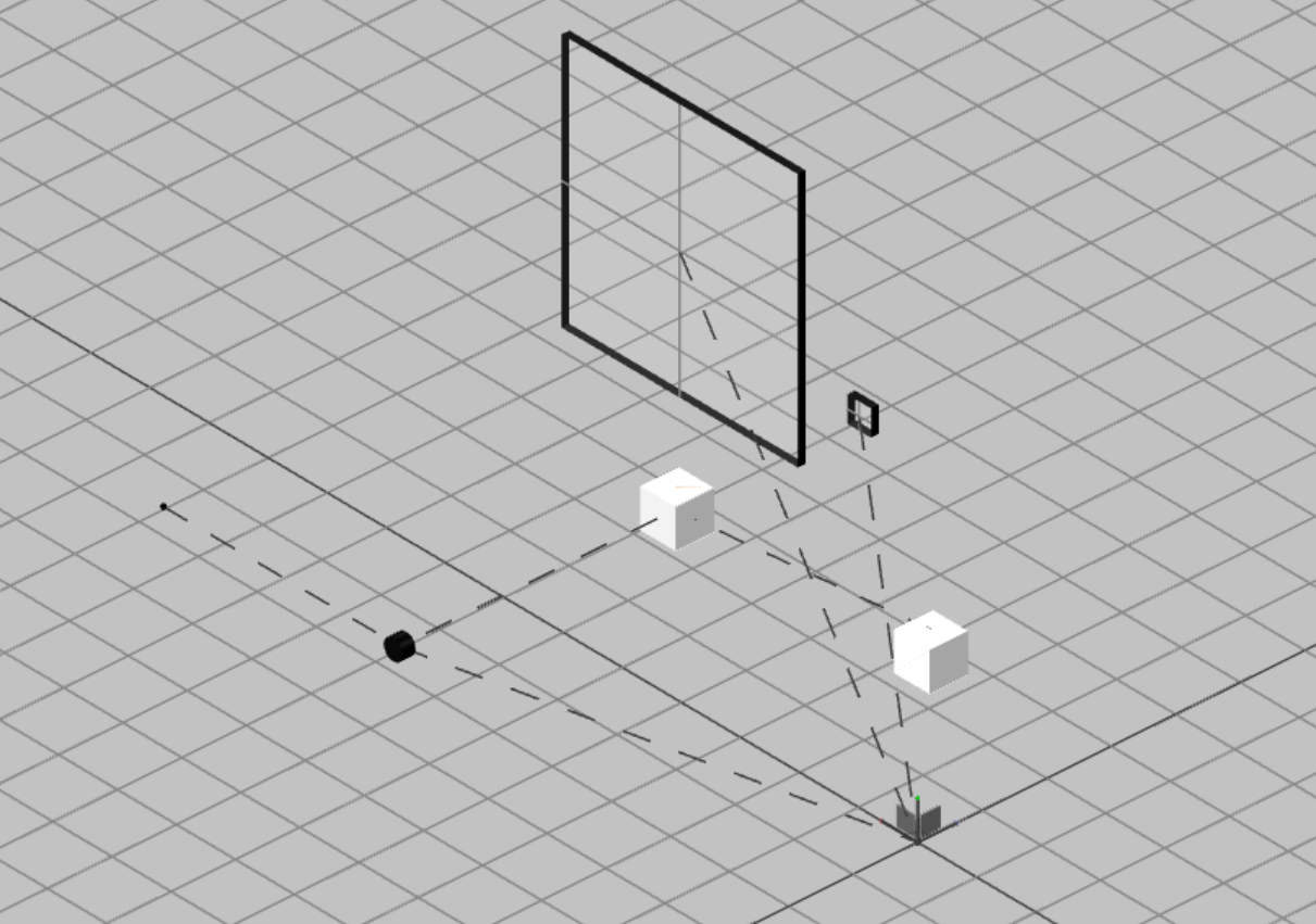
After selecting an element on the layout or the Outliner, click the button on the right toolbar to open the Move/Rotate dialog box. The selected element's position is displayed relative to the specific coordinate system which is marked by the dotted line on the layout. Note: Each element is created with a location relative to the global coordinate system (GCS), as in the example below. Manually change the values (position in mm/ inches, angle in degrees/mrad) to move the element, or drag it and the location values are updated.
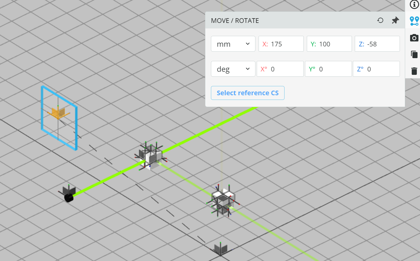
To locate the element relative to another element, click Select reference CS in the dialog box. At this stage, all available LCSs will be displayed in the layout.
You can select any element by left-clicking on the layout, or selecting it in the Outliner. After selecting the LCS, the values will update automatically. You can now adjust the position of the element by manually changing the appropriate values in the dialog box.
By clicking on the upper toolbar, you can see the linkage of every element to its LCS with dotted lines.
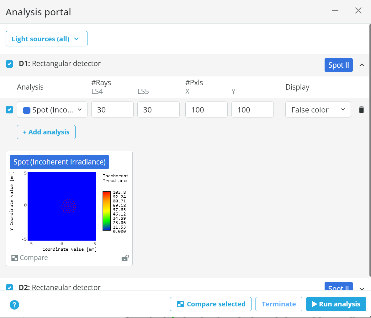
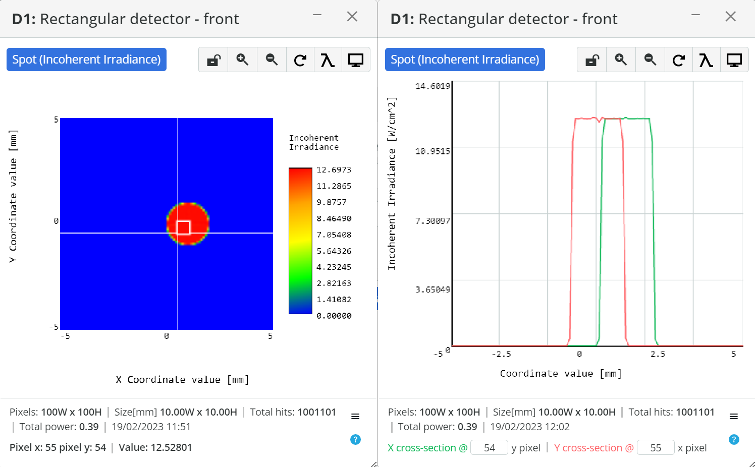
Click to open the Analysis Portal. It includes all the setup’s detectors and light sources, and by default a single analysis per detector: fast incoherent spot.
All the fast analyses can be presented and positioned on a layout view by clicking .
Click on a detector line to open the analysis results.
Notes:
Using the Analysis Portal
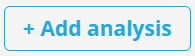
Click to add an analysis for a specific detector. By default it is added as a fast incoherent spot which can be changed to a different advanced analysis: incoherent or coherent spot, and coherent phase. You can use more than one analysis per detector for comparison .
activates by default, or deactivates a specific analysis that has been run
deletes the selected analysis from the specific detector.
The differences between fast and advanced analyses are:
|
|
Fast |
Advanced |
|
Max. number of pixels |
100 x 100 |
3,000 x 3,000 |
|
Max. number of rays per light source. |
200 |
Unlimited |
|
Spot (incoherent irradiance) |
Yes |
Yes |
|
Spot (coherent irradiance) |
No |
Yes |
|
Coherent phase |
No |
Yes |
Click to start the analysis. You can also click the layout ray tracing ‘Propagation simulation button.
Click to terminate the analysis before it has been completed.
Click to run a comparative analysis. Select the analyses by clicking in the bottom left corner of each analysis.
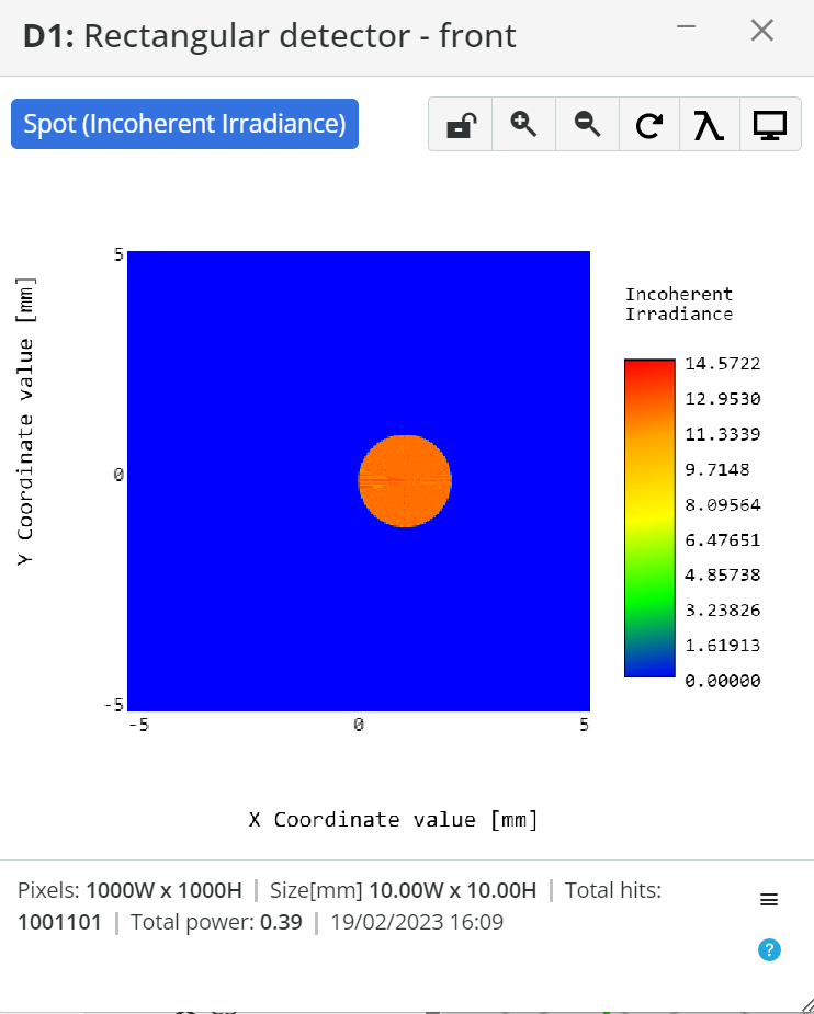
Click on each of the analysis results to open it in the extended view, which provides you with additional data inputs and analysis features.
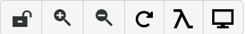
Toolbar Description
There is a toolbar in the top right corner:
Lock/unlock chart: Used for comparison so that the original configuration result can be “frozen” and compared to additional configurations based on changes to the setup.
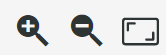
Zoom in/out: You can also left click and select an area to zoom in.
Reset to the original zoom
Present data for all wavelengths or the selected ones only.
Change the display type:
is located in the bottom right corner of the analysis extended view. Click it for the following features: